Pharmacokinetics (PK) describes what the body does to a drug. It draws on in vivo studies in preclinical animals as well as studies in human subjects. During drug development, ADME studies are designed to predict the properties of a therapeutic candidate and assess its suitability for further development. The links between in vivo and in vitro PK properties are often unclear. As a result, physiologically based pharmacokinetics emerged to provide a formal connection between the in vitro biochemical realm and in vivo, bioanalytically measurable descriptors. This is a basic sheet of terms for scientists who are new to pharmacology.
1. Basic in vivo PK properties
Dose is the total amount of drug injected into an organism.
t1/2 – half-life of the molecule – the time needed to eliminate 50% of the molecule from the body. The concept comes from the general first-order kinetic approximation, in which the half-life does not depend on the initial concentration. Because this assumption is not fully met in living systems, this definition can be ambiguous.
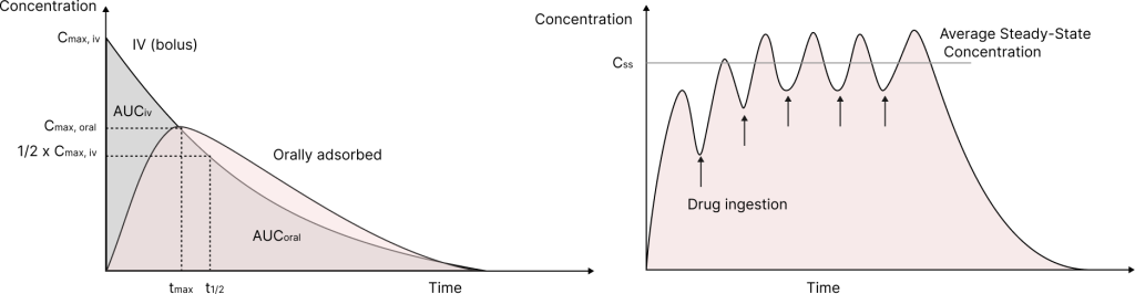
Plasma concentration – time curve generalises the evolution of drug concentration in plasma, which often correlates with concentrations in tissue reservoirs. Therefore, we can assume that plasma concentration is proportional to the degree of response.
Cmax is the maximum concentration of the drug in plasma achieved during a single drug injection. For an intravenous bolus injection, Cmax is achieved at t=0. In other cases, it is achieved at t=tmax after injection.
The integral over the concentration-time curve is defined as the Area under the curve (AUC). This value is proportional to the amount of drug distributed in the organism.
Upon multiple drug applications, the plasma concentration – time curve oscillates between the minimum and maximum concentrations. When the oscillations become approximately constant and periodic, a steady state is achieved. The average concentration of the drug at steady state is an essential value for further PK studies (Css,av).
2. Bioavailability
Bioavailability (F) is defined as the total amount of drug reaching the bloodstream and tissue reservoirs, and can be determined as
F = AUC iv / AUC oral
In mechanistic definitions, it can be described as follows:
F oral = Fa x Fg x Fh = Fa x (1 – Eg) x (1 – Eh)
Where Fa – fraction of dose adsorbed into the intestinal wall, Fg – fraction of dose released by the intestinal wall into the bloodstream, Fh – fraction of drug not adsorbed by the liver during the first pass, Eg – gut extraction ratio, Eh – liver extraction ratio.
Fa can be determined using conventional permeability assays (Caco-2 or MDCK cell line-based assays). Fg summarises non-specific binding in the intestine and metabolism by intestinal enzymes. For most **Rule of 5-**compliant molecules, Fg = 1. However, most currently developed molecules have Fg < 1 and require investigation with enterocyte-derived cellular or subcellular models. The Fh = 1 – Eh term is determined from the well-established ratio
Eh = CLh / Q
Where CLh is hepatic clearance and Q is portal vein blood flow.
3. Distribution
Drug distribution through the body is determined by the equilibrium of exchange between plasma and a tissue reservoir. We assume that only free drug (Cfree) can travel through the endothelium into tissue and determine drug action (”free drug hypothesis”). In plasma, the drug is partially bound by proteins such as albumin or lipoproteins. Therefore, the free drug concentration is determined as
Cfree = fub,p * Ctotal
Where Ctotal – the total amount of drug that reached the bloodstream, and fub,p – an unbound fraction of a drug in plasma that is constant during equilibrium.
fub = Cfree/(Cfree + Cbound) = Cu/(Cu + Cu x [P] x n x Kb) = 1 / (1 + [P] x n x Kb) = const
Where Cb – concentration of drug bound to protein, [P] – equilibrium concentration of proteins in plasma, Kb – binding constant, n – number of binding sites on the protein surface.
Some compounds have significant absorption into erythrocytes. Therefore, a factor such as the blood-to-plasma ratio (R) can be determined as follows:
R = (Ce x H + Cp x (1 – H))/Cp
Where Ce – concentration of drug in erythrocytes, H – hematocrit, Cp – total concentration of drug in plasma.
Since we consider distribution to be guided by a quasi-equilibrium exchange process, we can consider the following scheme:
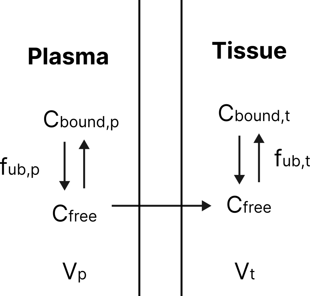
Where Vp – volume of plasma, Vt – volume of the tissue reservoir, fub,t – unbound fraction in tissue
If we introduce the value Vd, it represents the imaginary volume in which the drug at concentration Cp distributes, conserving mass balance. Its definition is as follows:
Vd x Cp = Vp x Cp + Vt x Ct
Vd = Vp + Vt x Ct / Cp = Vp + fub,p / fub,t * Vt
In this definition, we transition from unmeasurable Cbound and Cfree values to measurable fub terms. Distribution volume (Vd) determines the affinity of a drug for tissue reservoirs compared to plasma binding.
This parameter can also be directly connected to in vivo data:
Vd = (Dose x F)/Cp
In steady state, the same applies:
Vss = (Abss)/Css
Where Vss – volume of distribution in steady state, Abss – total amount of drug absorbed in steady state.
4. Clearance
Clearance ([volume/time] units) is a theoretical property of a drug molecule that determines the volume of plasma cleared of the drug per unit of time. In more practical terms, it is the component of total plasma flow that does not contain the drug. This flow formalism allows the individual organ clearance values to be summed. For a typical small molecule, clearance can be determined as
CL = CLh + CLr + …
Where CLh – hepatic clearance, CLr – renal clearance, CL – total clearance.
From the other side:
CL = Dose/AUC
It is difficult to measure an individual organ clearance, so in vitro ADME studies are useful here. Since clearance in the liver is highly compound-dependent and cannot be extrapolated from historical data, hepatocyte and microsomal assays are crucial. To integrate in vitro findings and in vivo measurements, two major approaches exist. First, compound flow models predict CLh from CLint (intrinsic clearance in vitro) by scaling measured in vitro data. One such model, and the most popular one, is the well-stirred reactor model, which approximates liver absorption as a fast mass-transfer reactor.
CLh = Q x fub,p x Clint/(Q + fub,p x Clint)
Q – flow of blood through the liver
This model determines that at high Clint (high-clearance compounds, Eh > 70%)
CLh —> Q
At low Clint (low-clearance compounds, Eh < 30%)
CLh —> Clint x fub,p
However, this approach can deviate substantially from the actual CL for both high- and low-clearance compounds, due to the fundamental nature of its assumptions.
Therefore, the physiologically-based pharmacokinetics differential-equation formalism is more faithful, but it does not allow robust simplifications. It includes Michaelis-Menten approximations for uptake, metabolism, and efflux to generate CLh from first principles.
For in vitro measurements, two approaches exist, following basic Michaelis-Menten conclusions. Since Km for Phase I and Phase II metabolism processes exists in the range from 50 uM to 200 uM, at [S] << Km
d[P]/dt = Vmax x [S] / Km = kel x [S]
Where kel – elimination rate constant. Then we can determine Clint as
Clint = kel/(concentration of metabolising cells/protein) [volume/min/number of cells or volume/min/mg of protein]
Then we can scale up Clint to the whole organ, knowing number of cells/protein in liver.
We can also operate in activity terms at [S] >> Km. Then
A = Vmax/(concentration of metabolising cells/protein) [number of moles/min/number of cells or number of moles/min/mg of protein]
Clr can be approximated from the glomerular filtration rate (GFR) in the simplified approach, and similarly using PBPK simulation using a three-compartment model (Renal Interstitial, Proximal tubule cell, Proximal tubule lumen).
By analogy to F, biliary excretion can be estimated using the Biliary Excretion Index (BEI), a percentage of the drug adsorbed into bile from the total amount. However, this static value poorly translates into in vivo findings. Therefore, the kinetic Km and Vmax formalism is used during PBPK modeling, and both can be estimated from in vitro studies.
Most definitions for time-dependent processes exist in two forms:
- scalable quasi-first- or quasi-zero-order clearance values
- complete PBPK Michaelis–Menten definitions.
Across teams’ experiences, the first set is sometimes not directly translatable to in vivo findings; however, the second can be cumbersome and difficult to interpret outside the differential-equation framework. Further studies are needed to derive robust in vitro-to-in vivo translation models across a wide range of compounds.
Explore our new ADME products brochure.
Written by Anton Hanopolskyi